| decision | series | why | |
|---|---|---|---|
| 0 | tradable (rank & hold) | SPY | investable channel proxy |
| 1 | tradable (rank & hold) | XLE | investable channel proxy |
| 2 | tradable (rank & hold) | ITA | investable channel proxy |
| 3 | tradable (rank & hold) | DBA | investable channel proxy |
| 4 | tradable (rank & hold) | BDRY | investable channel proxy |
| 5 | tradable (rank & hold) | GLD | investable channel proxy |
| 6 | tradable (rank & hold) | UUP | investable channel proxy |
| 7 | tradable (rank & hold) | BTC-USD | investable channel proxy |
| 8 | tradable (rank & hold) | ETH-USD | investable channel proxy |
| 9 | tradable (rank & hold) | LMT | investable channel proxy |
| 10 | tradable (rank & hold) | COPPER | investable channel proxy |
| 11 | regime / macro input | BAA10Y / NFCI / curve | gates gross exposure / routes channels |
| 12 | regime / macro input | T10YIE / DFII10 | reflation-vs-stagflation quadrant |
| 13 | regime / macro input | ICSA / PERMIT / … | leading-indicator block → diffusion-LEI |
| 14 | dropped — duplicate | VIXCLS | ≈ ^VIX (kept VIX) |
| 15 | dropped — duplicate | EIA_WTI | ≈ FRED WTI (kept DCOILWTICO) |
| 16 | dropped — duplicate | EURUSD_AV | ≈ Treasury EUR (kept for FX level) |
4 Data Preparation
CRISP-DM Phase 3. Construct the final dataset fed to the modeling tools — select, clean, construct (feature-engineer), integrate, and format. Usually the most time-consuming phase. See The CRISP-DM Process for the overview.
This chapter executes CRISP-DM Phase 3 for PortfolioLens. It picks up the Data Understanding hand-off — a ranked set of highest-value indicators (§5.1 there) and the explicit steer that, in a ~9-proxy universe, “which assets rise most” is a risk-adjusted, two-layer problem — and turns the raw snapshot into a leakage-aware, stationary feature matrix.
All logic lives in scripts/poc_prepare.py (the chapter stays thin, mirroring poc_quality.py); every cell reads only the committed snapshot — no live API calls, no keys. The design follows the Indicator Council’s two rulings: features are constructed here, not in Phase 2, and the model’s target is risk-adjusted forward return, never raw “largest increases.”
4.1 1. Select data
We keep the buyable proxies (the assets a model would rank and the portfolio could hold) plus the regime/macro inputs that gate exposure. Three snapshot series are demonstration / cross-check duplicates and are dropped from the feature build:
^VIX is itself not investable, so it is a regime input only — excluded from the tradable ranking layer even though it stays in the feature set as a volatility gauge.
4.2 2. Clean data
Three Phase-2 quality findings (§7) dictate the cleaning rules:
- Negative WTI (April 2020). A real print that breaks log math — so WTI is used only via levels/changes, never log-returns, and is not a tradable in the ranking layer.
- Calendar misalignment. Crypto trades 7 days/week, equities ~5, NFCI weekly, macro monthly. We resample everything onto a business-day master calendar.
- Release lag / look-ahead. Monthly/weekly macro is stamped by reference period but known only on the later release date, so
prep.align_featureslags each release to its publication date before forward-filling it as a step function — never across the frontier.
fig, ax = plt.subplots(figsize=(10, 3.8))
raw = panel["UMCSENT"].dropna()
ax.plot(raw.index, raw, "o", ms=2.5, color="tab:gray", label="raw monthly print (reference date)")
ax.plot(aligned.index, aligned["UMCSENT"], color="tab:blue", lw=1.0,
        label="lag-aware, business-day step")
ax.set_xlim(pd.Timestamp("2018-01-01"), pd.Timestamp("2021-06-01"))
ax.set_ylabel("UMich sentiment")
ax.set_title("Release-lagged, forward-filled alignment (zoom)")
ax.legend(loc="lower left", fontsize=8)
plt.tight_layout()
plt.show()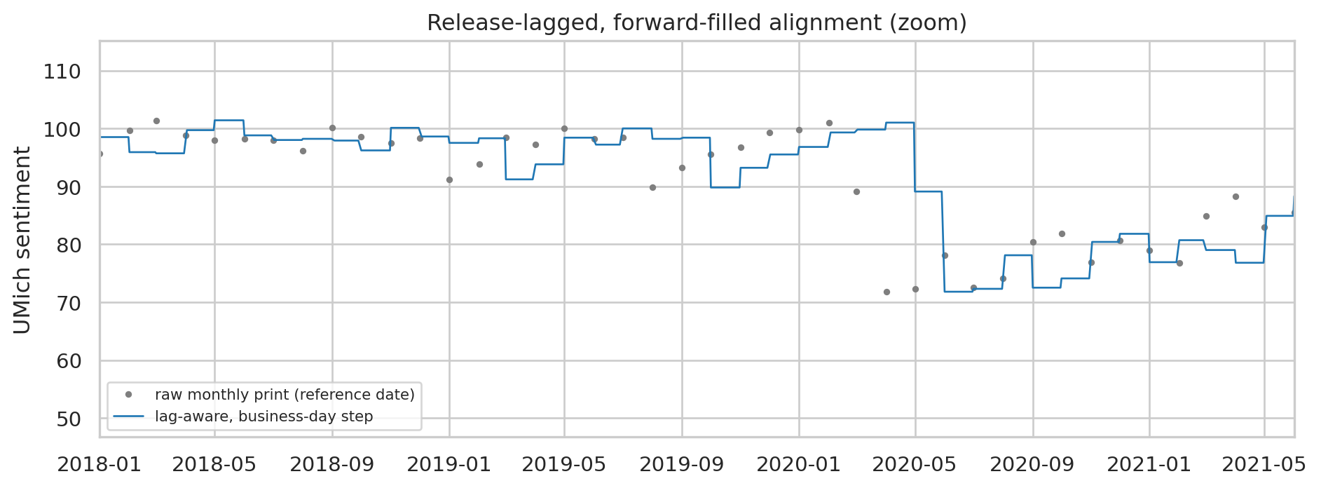
4.3 3. Construct data — the two-layer feature set
The highest-value indicators from §5.1 become features here. Layer A ranks which proxy leads; Layer B gates how much to hold.
4.3.1 3.1 Layer A — return ranking: volatility-scaled momentum
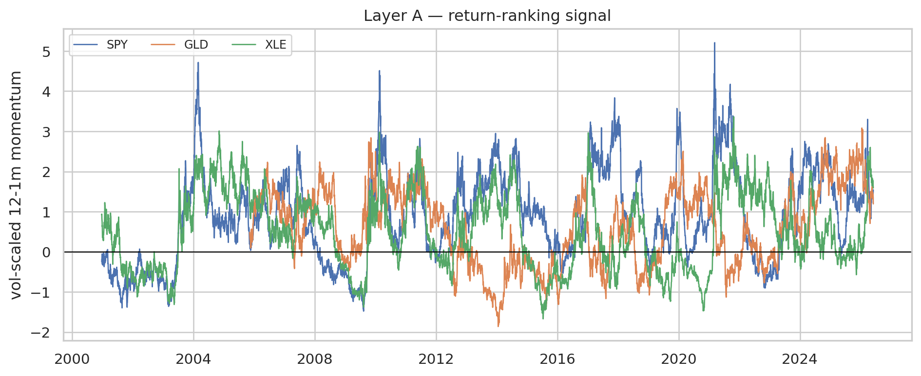
12-1 month momentum (skip the last month to avoid short-term reversal), divided by trailing volatility to tame the momentum-crash failure mode. A cross-sectional rank turns it into “who leads today”:
mom = prep.momentum(aligned[TRADABLE])           # vol-scaled 12-1m
rank = prep.cross_sectional_rank(mom)            # [0,1] within each date
latest = pd.DataFrame({"vol_scaled_momentum": mom.iloc[-1],
                       "cross_sectional_rank": rank.iloc[-1]}).sort_values(
                       "cross_sectional_rank", ascending=False).round(3)
latest| vol_scaled_momentum | cross_sectional_rank | |
|---|---|---|
| BDRY | 2.298 | 1.000 |
| XLE | 1.588 | 0.909 |
| SPY | 1.541 | 0.818 |
| GLD | 1.192 | 0.727 |
| COPPER | 0.800 | 0.636 |
| UUP | 0.796 | 0.545 |
| DBA | 0.779 | 0.455 |
| ITA | 0.748 | 0.364 |
| LMT | 0.366 | 0.273 |
| ETH-USD | -0.192 | 0.182 |
| BTC-USD | -0.735 | 0.091 |
4.3.2 3.2 Layer B — the equal-weighted regime score (gross-exposure dial)
Per the council’s anti-overfitting steer, the regime layer is a small, fixed, equal-weighted diffusion vote — no fitted weights — over robust stress signals (credit spread, curve inversion, financial conditions, Sahm, VIX). Its output is a gross-exposure multiplier, not a buy/sell trigger.
reg = prep.regime_score(aligned)
fig, ax1 = plt.subplots(figsize=(10, 4.2))
ax1.fill_between(reg.index, reg["regime_score"], color="tab:red", alpha=0.35,
                 label="regime score (0 calm → 1 stress)")
ax1.set_ylabel("regime score", color="tab:red")
ax2 = ax1.twinx()
ax2.plot(reg.index, reg["gross_exposure_dial"], color="tab:blue", lw=1.0,
         label="gross-exposure dial")
ax2.set_ylabel("gross-exposure dial", color="tab:blue")
ax1.set_title("Layer B — regime / exposure gate")
plt.tight_layout()
plt.show()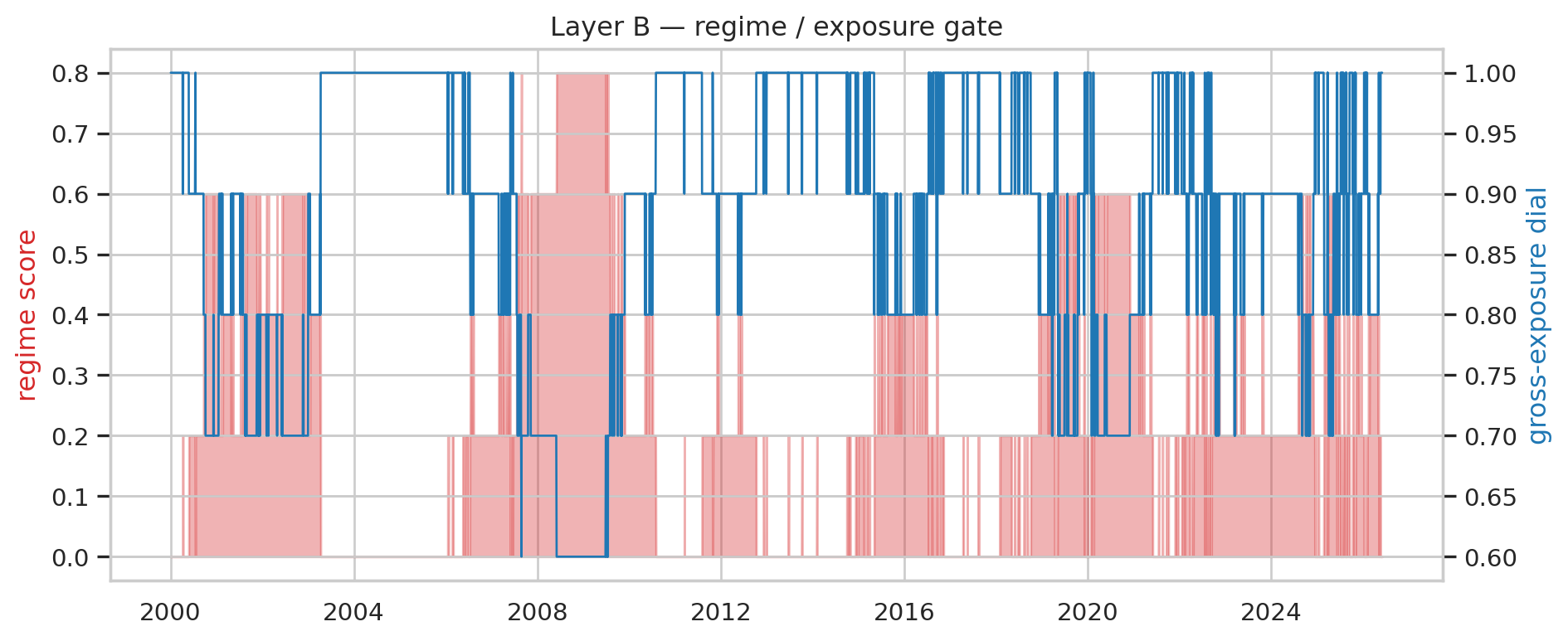
4.3.3 3.3 Channel routing — quadrant, copper/gold, and the diffusion-LEI proxy
The reflation/stagflation quadrant (breakevens vs real yields) routes the conflict-sensitive sleeve; copper/gold is the growth barometer; and the new free leading-indicator block powers a homemade diffusion-LEI (share of LEI components rising over ~6 months) — a free stand-in for the licensed Conference-Board index.
Quadrant distribution (business-days):
quadrant
overheat                1661
reflation               1598
goldilocks              1575
deflation/tightening    1212

Diffusion-LEI components available: 7 of 7
Latest diffusion-LEI (share rising): 0.86
Latest copper/gold z-score: -0.40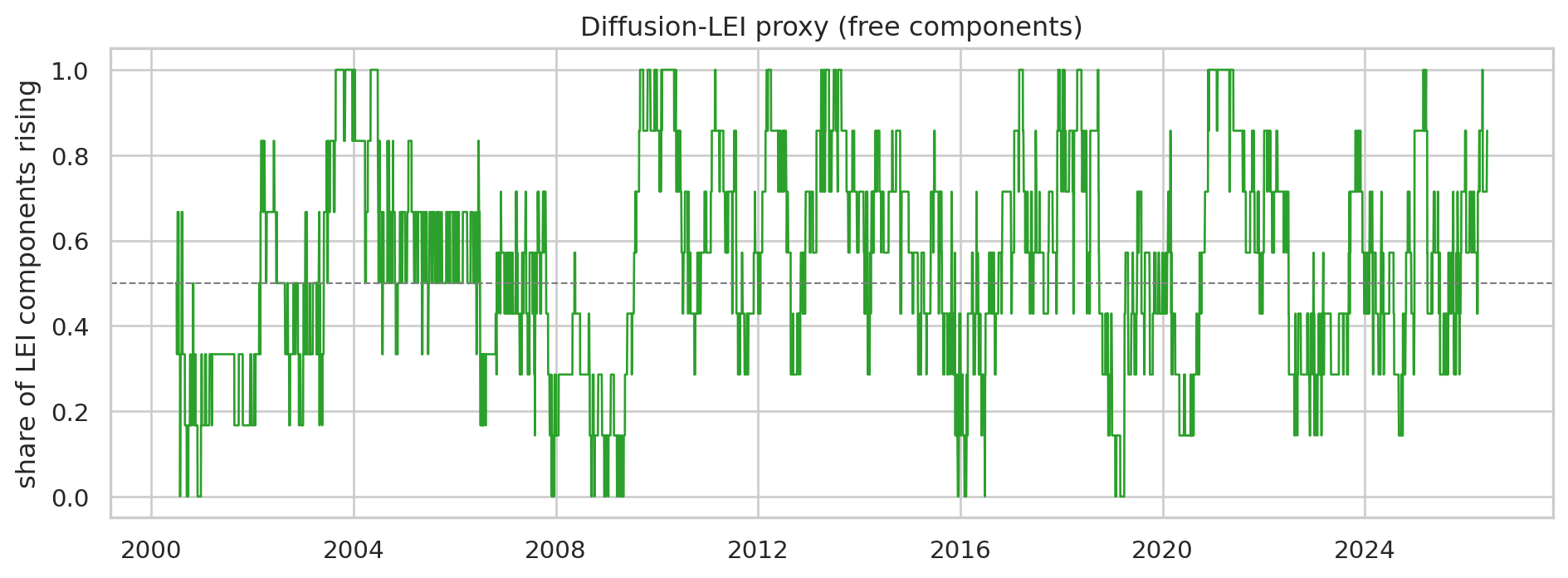
4.4 4. Integrate & format — the modeling matrix
prep.build_feature_matrix joins every feature onto the business-day master and builds the labels separately: the target is forward return ÷ trailing volatility (risk-adjusted, multi-horizon), kept strictly apart from the features so the look-ahead in the label can never leak into X.
X, Y = prep.build_feature_matrix(SNAP)
print(f"Features X : {X.shape[0]} business days, {X.shape[1]} columns")
print(f"Labels   Y : {Y.shape[1]} columns (forward risk-adjusted return, 21d & 63d)")
print("\nFeature columns:")
print(", ".join(X.columns))
Features X : 6892 business days, 38 columns
Labels Y : 22 columns (forward risk-adjusted return, 21d & 63d)
Feature columns:
mom_SPY, momrank_SPY, mom_XLE, momrank_XLE, mom_ITA, momrank_ITA, mom_DBA, momrank_DBA, mom_BDRY, momrank_BDRY, mom_GLD, momrank_GLD, mom_UUP, momrank_UUP, mom_BTC-USD, momrank_BTC-USD, mom_ETH-USD, momrank_ETH-USD, mom_LMT, momrank_LMT, mom_COPPER, momrank_COPPER, regime_score, gross_exposure_dial, curve_10y2y, curve_10y3m, BAA10Y_z, NFCI_z, ANFCI_z, VIX_z, sahm_flag, breakeven_chg_3m, realrate_chg_3m, quadrant, copper_gold, copper_gold_z, lei_diffusion, lei_n_components| mom_SPY | momrank_SPY | mom_XLE | momrank_XLE | mom_ITA | momrank_ITA | mom_DBA | momrank_DBA | mom_BDRY | momrank_BDRY | mom_GLD | momrank_GLD | mom_UUP | momrank_UUP | mom_BTC-USD | momrank_BTC-USD | mom_ETH-USD | momrank_ETH-USD | mom_LMT | momrank_LMT | mom_COPPER | momrank_COPPER | regime_score | gross_exposure_dial | curve_10y2y | curve_10y3m | BAA10Y_z | NFCI_z | ANFCI_z | VIX_z | sahm_flag | breakeven_chg_3m | realrate_chg_3m | quadrant | copper_gold | copper_gold_z | lei_diffusion | lei_n_components | |
|---|---|---|---|---|---|---|---|---|---|---|---|---|---|---|---|---|---|---|---|---|---|---|---|---|---|---|---|---|---|---|---|---|---|---|---|---|---|---|
| 2026-05-29 | 1.474 | 0.818 | 1.754 | 0.909 | 0.819 | 0.545 | 0.648 | 0.364 | 2.362 | 1.0 | 1.431 | 0.727 | 0.632 | 0.273 | -0.895 | 0.091 | -0.396 | 0.182 | 0.667 | 0.455 | 0.917 | 0.636 | 0.0 | 1.0 | 0.47 | 0.76 | -0.649 | -0.829 | 0.049 | -0.424 | 0.0 | 0.09 | 0.30 | overheat | 0.015 | -0.706 | 0.714 | 7 |
| 2026-06-01 | 1.468 | 0.818 | 1.640 | 0.909 | 0.792 | 0.455 | 0.690 | 0.364 | 2.358 | 1.0 | 1.358 | 0.727 | 0.794 | 0.545 | -0.835 | 0.091 | -0.300 | 0.182 | 0.482 | 0.273 | 0.890 | 0.636 | 0.0 | 1.0 | 0.42 | 0.69 | -0.859 | -0.827 | 0.052 | -0.262 | 0.0 | 0.11 | 0.27 | overheat | 0.016 | -0.495 | 0.857 | 7 |
| 2026-06-02 | 1.541 | 0.818 | 1.588 | 0.909 | 0.748 | 0.364 | 0.779 | 0.455 | 2.298 | 1.0 | 1.192 | 0.727 | 0.796 | 0.545 | -0.735 | 0.091 | -0.192 | 0.182 | 0.366 | 0.273 | 0.800 | 0.636 | 0.0 | 1.0 | 0.41 | 0.69 | -0.857 | -0.826 | 0.055 | -0.325 | 0.0 | 0.08 | 0.25 | overheat | 0.016 | -0.398 | 0.857 | 7 |
Wrote 6892 rows x 60 cols -> data/prepared/feature_matrix.parquetThe matrix is persisted to data/prepared/feature_matrix.parquet (committed, like the snapshot) so Phase 4 can train without re-running this phase.
4.5 5. Honesty & anti-overfitting (Phase 4 hand-off)
The data forces discipline the Advisory Council and strategy.md §8 insisted on:
- Leakage control. Macro is publication-lagged before any fill; the forward-return label is the only deliberately look-ahead object and is never a feature.
- No fitted weights in the regime layer. With only ~3–4 genuine regimes in 25 years, an equal-weighted diffusion vote is more honest than estimated coefficients.
- Validation plan. Phase 4 must use purged/embargoed walk-forward CV, deflated Sharpe, and elevated t-stat hurdles, and benchmark against dumb buy-and-hold SPY and 60/40 — geopolitical/feature lift must beat the baseline out of sample.
- Still revised, not vintage. This PoC uses revised FRED; true point-in-time (ALFRED) vintages remain the Phase-3-to-4 upgrade. → Modeling.
Phase-3 deliverables — complete: data selection (§1), cleaning rules (§2), the two-layer feature construction realizing the §5.1 highest-value indicators (§3), and an integrated, formatted, persisted feature matrix with a risk-adjusted target (§4) — built entirely from the committed snapshot, with the reasoning recorded in the Indicator Council appendix.